
Secret tricks for using the VLOOKUP function with multiple criteria

Ngọc Phương
26-08-2021 . 960 view
The VLOOKUP function in Excel does not differentiate between Office 2010, 2013, or 2016; as long as it's an Excel spreadsheet, this calculation function can be run. The VLOOKUP function assists users in searching for data within a table and outputs the related results that need to be displayed.
In a list with many rows (a large quantity) and many columns (a lot of information), you can't possibly sit and scroll to search for information for each individual. The VLOOKUP function will help you quickly and accurately find the content you need.
I. The VLOOKUP formula in Excel
The general formula of the VLOOKUP function is as follows:
=/+ Vlookup(lookup_value,table_array,col_index_num,[range_lookup])
In which:
- =/+: In Excel, when typing a formula in a cell, you must start with an "=" or "+" sign. Vlookup is the function name in Excel.
- lookup_value is the value used for searching.
- table_array is the list table containing the search value.
- col_index_num is the column number of the data that needs to be returned on the list table.
- [range_lookup] is the search range. There are two values: 1 corresponding to True for approximate match, and 0 corresponding to False for exact match.
An absolute search in Excel means that the value used to search must be an exact match in the list to produce a return result. A relative search means that the value used to search does not have to be an exact match; the return result will be the closest approximate value in the data table.
II. When should you use the VLOOKUP function?
Excel has many functions with different purposes. So, in what situations should you use the VLOOKUP function in Excel?
Firstly, you already have a data table with many rows and accompanying descriptions.
Secondly, you need to look up descriptive information in that data table.
Thus, if your issue is: "I need to find 'description a' of 'object A' in 'data table AaBb'", then you definitely must use the VLOOKUP function.
III. What should you keep in mind when using the VLOOKUP function?
To ensure accurate calculations and faster search operations, when using the VLOOKUP function in Excel, you need to be aware of a few things:
- The data value table (table_array) must be an absolute reference. Otherwise, when copying the formula to other search values, the results will be incorrect.
- The search value (lookup_value) must be in the first column of the lookup table (table_array).
- In the data table, numeric values must be stored as numbers.
- The data table should not contain duplicate results. To be sure, you can highlight the data range and then go to Data -> select Remove Duplicates. Duplicate information will be highlighted.
IV. Examples of practical applications of the VLOOKUP function in Excel
The following specific examples will help you understand how to use the VLOOKUP function to find data.
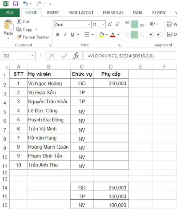
1. Example of calculating allowances for employees
In cell D2, use the VLOOKUP function to fill in the allowance for each different rank. Copy cell D2 and paste it into the remaining cells, and the results for everyone will be out.
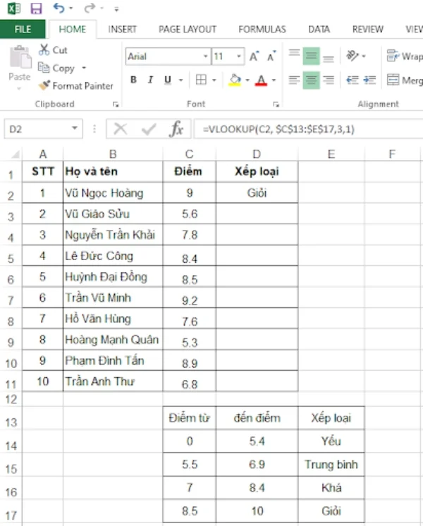
2. Example of relative search and grading of students
In cell D2, in the VLOOKUP formula, the position [range_lookup] is number 1 (approximate search) because many score values are not in the grading table. If changed to 0 (absolute search), the value will appear as #N/A.
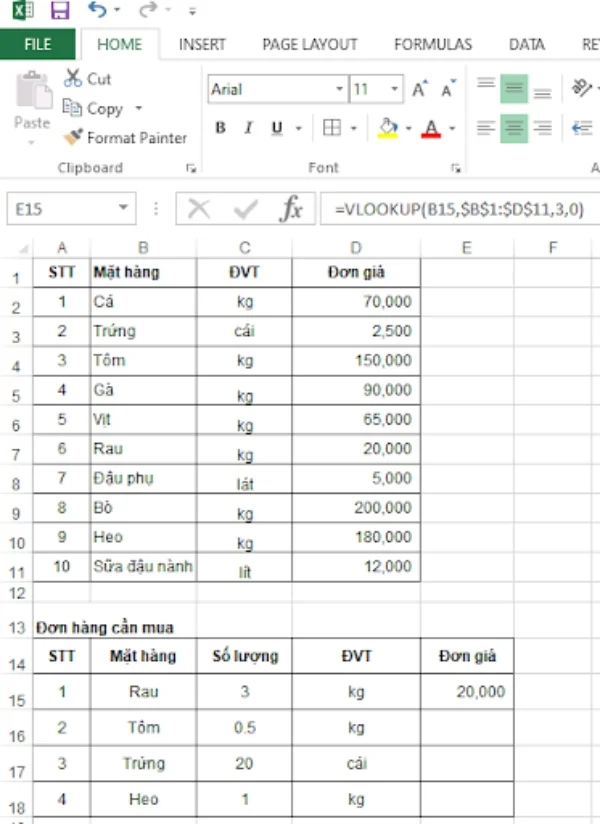
3. Example of extracting data
In cell E15, use VLOOKUP to find the unit price of the product according to the given price list.
V. Common errors when using the VLOOKUP function
Typing the VLOOKUP formula incorrectly will result in not finding the required result, and the system will display various error messages. Depending on the error symbol, we must review and correct the formula.
1. Error #N/A
This error occurs when the search value (lookup_value) is not found in the data table (table_array) or when the data return column (col_index_num) coincides with the column containing the search value.
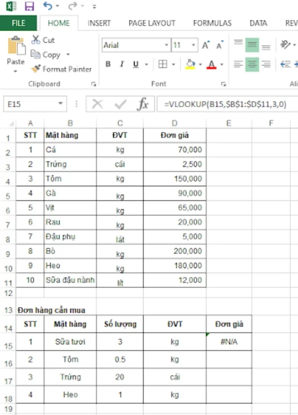
In cell E15, the product "Fresh Milk" is not in the price list, so the result shows #N/A.
2. Error #REF!
This error appears when the order number of the data return column (col_index_num) is not on the data table (table_array).
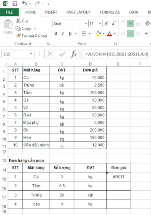
In cell E15, the data return column (col_index_num) is number 4, while the data table (table_array) $B$1:$D$11 has only 3 columns.
3. Error #VALUE!
This error occurs when you type the column order number of the data to be returned (col_index_num) as 0.
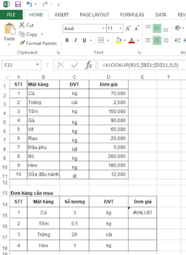
In cell E15, due to a mistake, the data return column (col_index_num) is entered as 0, so the result shows #VALUE!
4. Error #NAME?
This error often occurs when the lookup data (lookup_value) is in text format but is missing quotation marks.
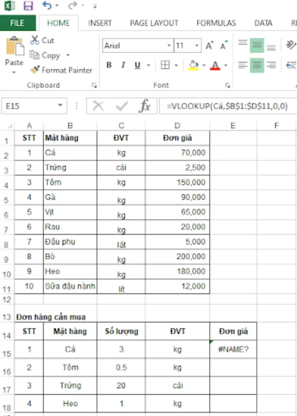
At cell E15, instead of entering the search data (lookup_value) as cell B15, you type in the word Fish, which results in the error #NAME?. If rewritten as "Fish," the result will be correct. However, in Excel calculations, it is better to use cell identifiers than text.
The VLOOKUP function in Excel may appear complex at first glance, but with some practice, you will understand how it works. Over time, you will be able to proficiently apply the formula to calculations, knowing when to use VLOOKUP, when to use If, Count, and other functions.
Ngọc Phương
Web Developer
Thank you for visiting my blog. My name is Phuong and I have more than 10 years of experience in website development. I am confident in asserting myself as an expert in creating impressive and effective websites. Anyone in need of website design can contact me via Zalo at 0935040740.
Submit feedback
Your email address will not be made public. Fields marked are required *
Search
Trend
-

The most commonly used HTML tags
02-01-2020 . 11k view
-

Websites for earning money at home by typing documents
05-17-2023 . 9k view
-

-

Earn money by answering surveys with Toluna
01-12-2020 . 7k view
-

Guide to creating a database in phpMyAdmin XAMPP
04-25-2020 . 4k view


0 feedback